Getting started
A first look at TransitionListener
Using TransitionListener for studying the gravitational wave signal from cosmological first-order phase transitions is really straightforward: Just run
$ tl -c examples/example_point.yaml -v
once you have installed TransitionListener and created a configuration file specifying the model parameters and desired outputs. For the example above, TransitionListener will create the following plot in the the folder scans/example_point/GW_spectrum.pdf:
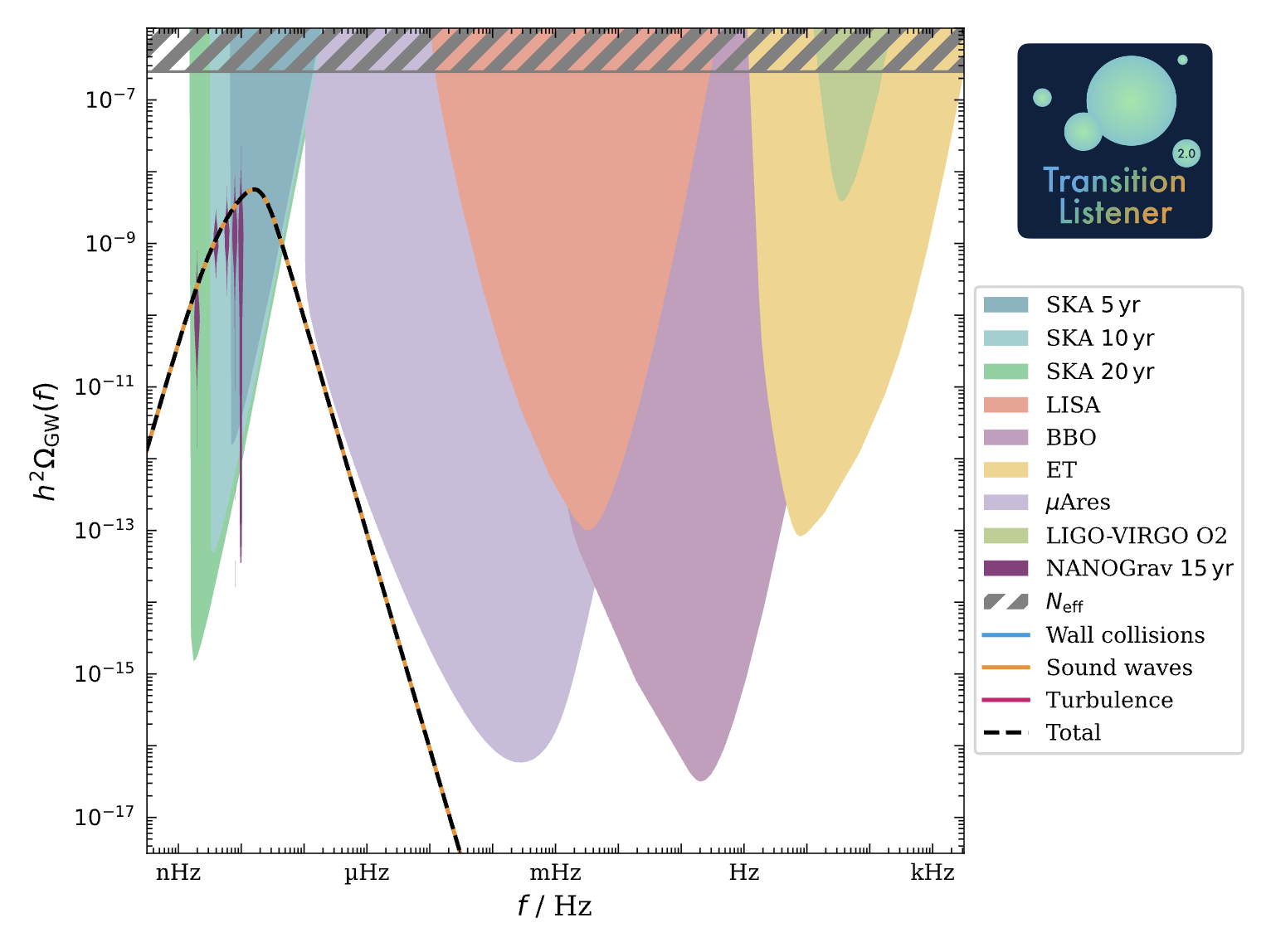
This is the gravitational wave spectrum produced by a first-order phase transition in a simple extension of the Standard Model with an additional U(1) gauge symmetry with conformal invariance, as described in arXiv:2502.19478.
Have a look into the configuration file examples/example_point.yaml. It starts as follows:
# This is an example yaml file

# ==================================================
# Scan settings
# ==================================================
Modelfile:
   models/TL_conformal_dark_u1.py

Scan:
   SinglePoint

Parameters:
   g: 0.7      # gauge coupling
   v_GeV: 0.1  # vacuum expectation value in GeV
   y: 0.01     # Yukawa coupling
Change the model input parameters to see how the gravitational wave signal is affected! You can also leave out the -v flag to suppress verbose output in the console.
More plots and diagnostics
Let’s discover the various options of the yaml` file for controlling TransitionListener. The yaml file continues as follows:
# ==================================================
# Output settings
# ==================================================
timeout: -1  # Timeout in seconds, -1 for no timeout
format: "txt"  # either "txt" or "hdf5"
output_path: "scans/example_point"
description: "example point, conformal U(1) model"
plot_description: "Example point, conformal $U(1)$ model"
This part specifies the output format and location as well as a timeout for the run. Sometimes, e.g., when working on a cluster with limited resources, it is useful to set a timeout for the run. The output format can be either .txt files or .hdf5 files. The output path specifies the folder where all output files will be stored. The description and plot_description fields are used for labeling the output files and plots. Note that the plot_description field supports fancy LaTeX formatting. 😊
The next part of the yaml file controls the plotting options:
# ==================================================
# Plot settings
# ==================================================
# Additional plotting options for single point scans
additional_plots:
   action:
      plot?: False
      Tmin_GeV: 0
      Tmax_GeV: 0.05
      phase_indices: [0, 1]
      n: 100

   potential:
      plot?: False
      T_GeV: 0.02
      phi_ranges_GeV: [0, 1]
      n: 100

   phases:
      plot?: False
      include_transitions?: False

   profileV:
      plot?: False
      field_index_1: 0
      field_index_2: 1

   energy_density:
      plot?: False
      Tmin_GeV: 0.01
      Tmax_GeV: 0.05

   dofs:
      Tmin_GeV: 0.01
      Tmax_GeV: 0.05
      plot?: False

   sensitivities:
      plot?: False

   profile:
      plot?: False

   percolation:
      plot?: False

   gw_spectrum:
      plot?: True
Each subsection under additional_plots toggles a specific figure via
its plot? flag and carries the configuration values needed for that plot.
Just try setting some of the plot? flags to True and re-run
TransitionListener to see the corresponding plots being created in the output
folder! If you want to learn more about the individual plots and their
configuration options, please refer to the Plots section of the
documentation.
That’s it! You are now ready to explore TransitionListener and its features. Have fun studying cosmological phase transitions and their gravitational wave signals!
For detailed installation instructions and usage examples please refer to the following sections:
Installation: Installation Guide
Usage: Usage
For more information, visit the documentation at https://tasillo.de/TransitionListener_development or check out the code repository at https://github.com/tasicarl/TransitionListener.