Example Output

This page collects representative TransitionListener output from published applications and from the shipped grid-scan example.

Published applications

TransitionListener has already been used in several dark sector and gravitational wave studies:

1. Turn up the volume: listening to phase transitions in hot dark sectors
   arXiv: 2109.06208, JCAP 02 (2022) 014.
   This work introduced the original TransitionListener workflow for a dark Abelian Higgs model and used it to compute phase-transition dynamics, dilution effects, and the resulting gravitational wave signal for hot dark sectors.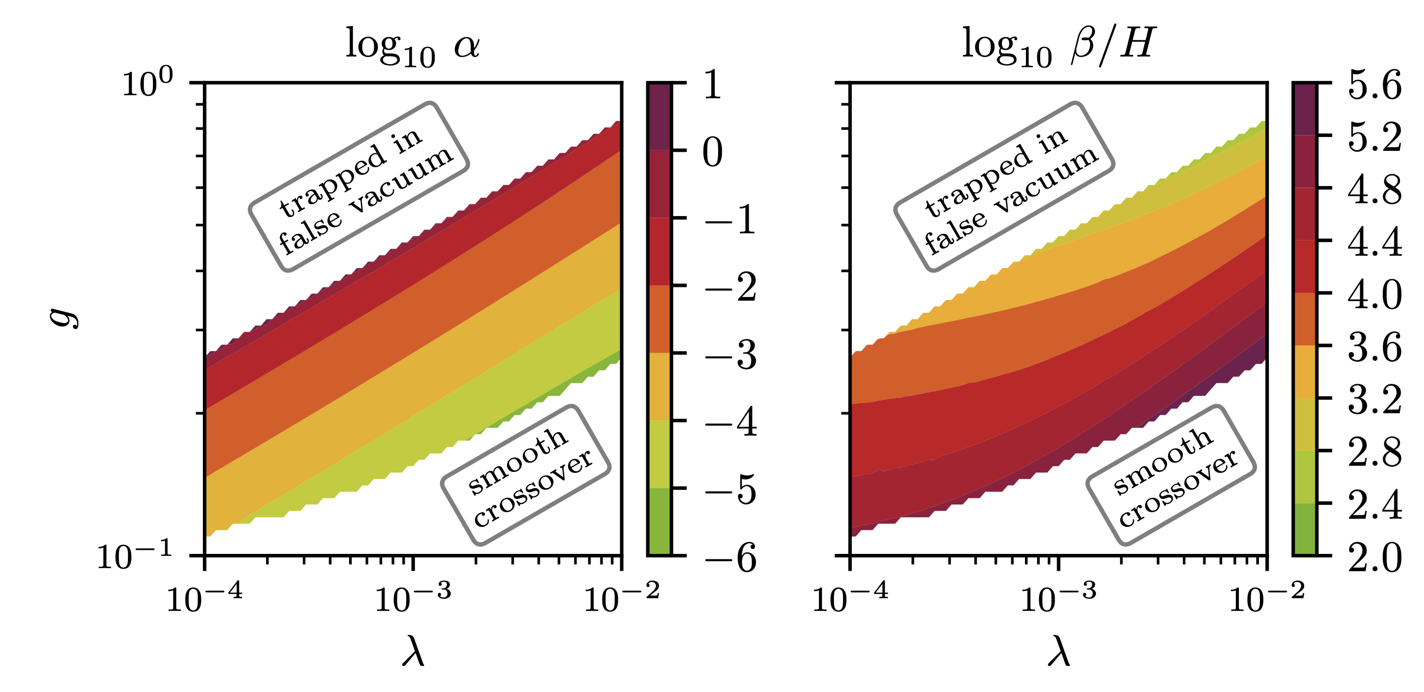

   

2. Hunting WIMPs with LISA: correlating dark matter and gravitational wave signals
   arXiv: 2311.06346, JCAP 05 (2024) 065.
   Here TransitionListener was used to map the phase-transition and gravitational wave predictions of a dark \(U(1)^\prime\) model onto the relic-density requirement, exposing the correlation between dark matter freeze-out and the milli-Hertz gravitational wave signal.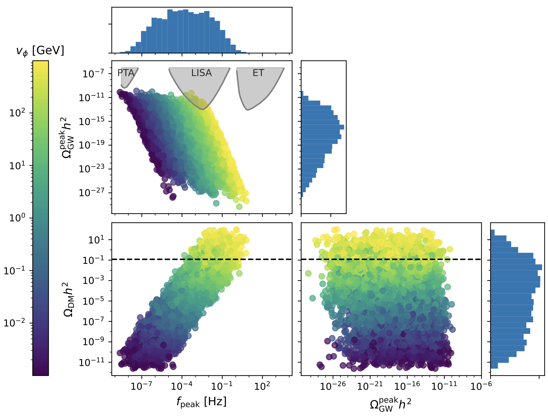

   

3. Sub-GeV dark matter and nano-Hertz gravitational waves from a classically conformal dark sector
   arXiv: 2502.19478, JCAP 08 (2025) 062.
   In this project TransitionListener was applied to a classically conformal dark \(U(1)^\prime\) model in order to identify parameter regions that simultaneously yield a PTA-scale gravitational wave signal, the observed dark matter abundance, and consistency with laboratory and cosmological constraints.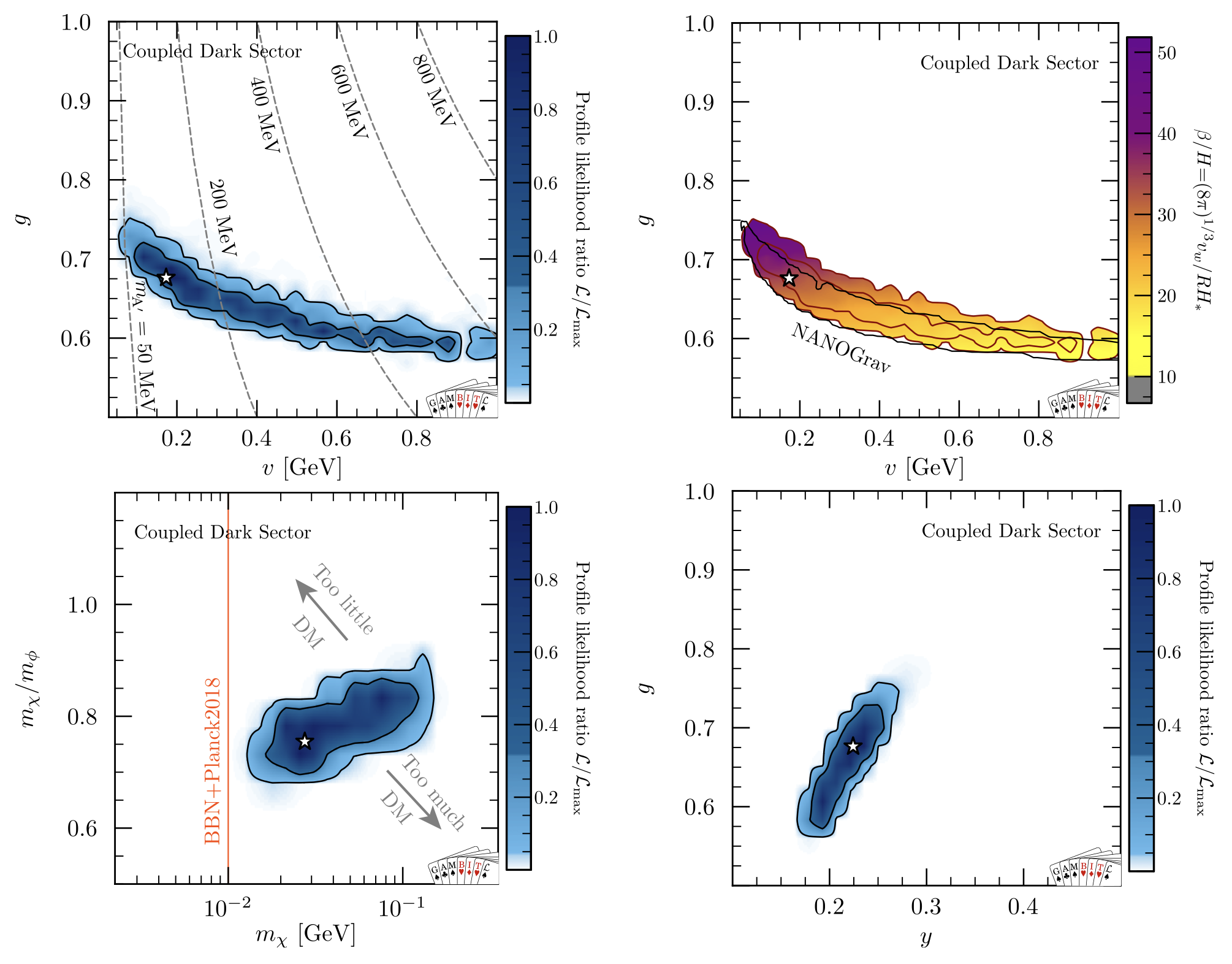

   

4. Tuning the violins: dark sector phase transition models for the PTA signal
   arXiv: 2602.09092.
   This study used TransitionListener random scans and its UltraNest/PTA-likelihood interface to compare several dark-sector model classes and quantify how much tuning is required to explain the PTA signal.

The following figure is the \(\alpha\)–\((\beta/H)_{RH}\) comparison plot discussed in the TransitionListener v2 paper and attributed there to the last study above:

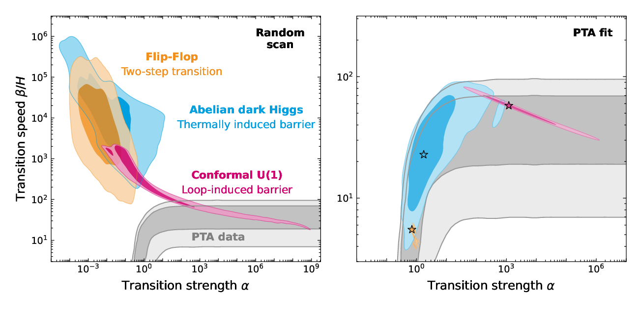
It compares three dark-sector model classes in the \(\alpha\)–\((\beta/H)_{RH}\) plane. The left panel shows generic model predictions from TransitionListener random scans, while the right panel shows the regions favored by PTA-informed nested sampling with the UltraNest backend.

Reproducing the shipped grid scan

The gallery below is generated from the example configuration examples/example_grid.yaml, which runs a grid scan of the Abelian dark Higgs model implemented in models/TL_dark_U1.py.

The scan settings are:

• x-axis parameter: l on a logarithmic grid from \(10^{-4}\) to \(10^{-2}\)

• y-axis parameter: v_GeV on a logarithmic grid from \(10^{6}\) to \(10^{10}\) GeV

• fixed input: g_tilde = 2.69

• precision preset: benchmark

• grid size: 10 x 10

Run it with:

tl -c examples/example_grid.yaml -j 10

The produced plots in scans/example_grid/ are then copied into the docs as PNG files for the gallery below.

Transition strength and milestone temperatures

These panels summarize how the transition strength and the characteristic temperatures vary across the two-dimensional parameter grid.

alpha	betaH_RH	Tcrit_SM_GeV	Tnuc_SM_GeV
Tperc_SM_GeV	Tf_SM_GeV	Treh_SM_GeV

Plasma and thermodynamic quantities

These plots expose the background-fluid quantities that enter the time-temperature relation and the macroscopic transition observables.

c_s_sym	c_s_bro	g_eff_tot_reh	xi_crit

Peak gravitational wave observables

These panels show the peak frequency and peak amplitude of the predicted gravitational wave spectrum across the scan.

log10_f_peak_Hz	log10_h2OmegaGW_peak

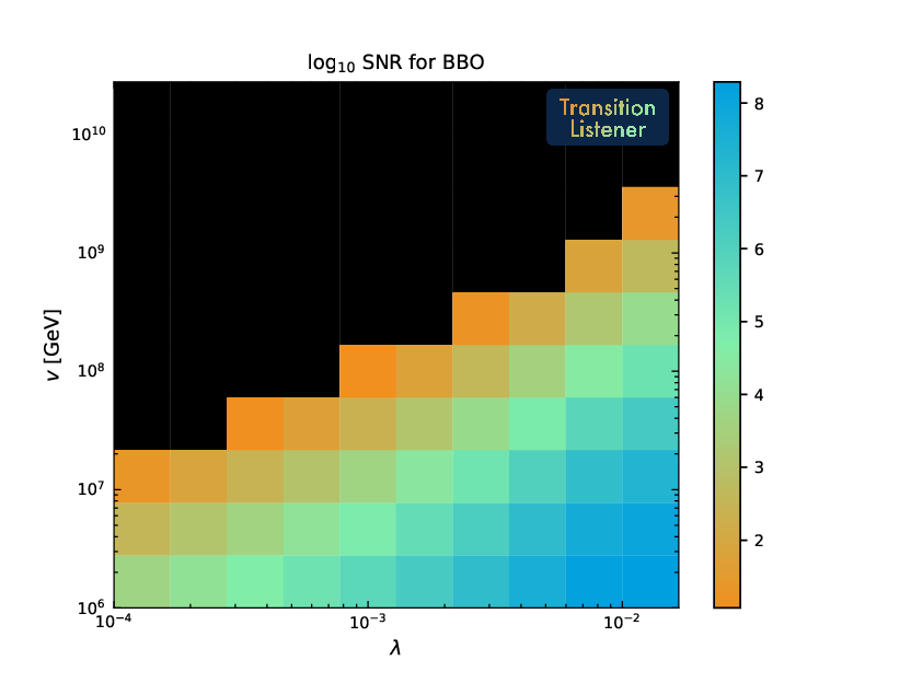
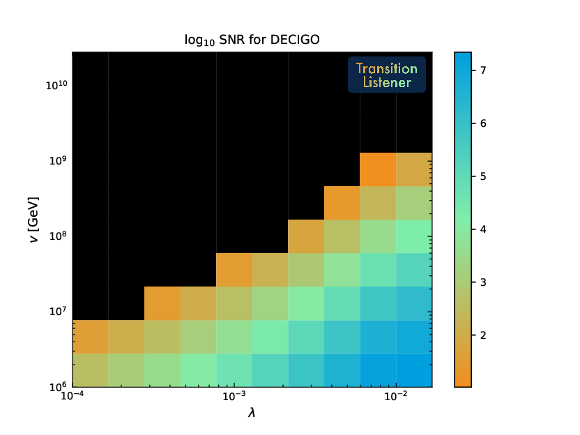
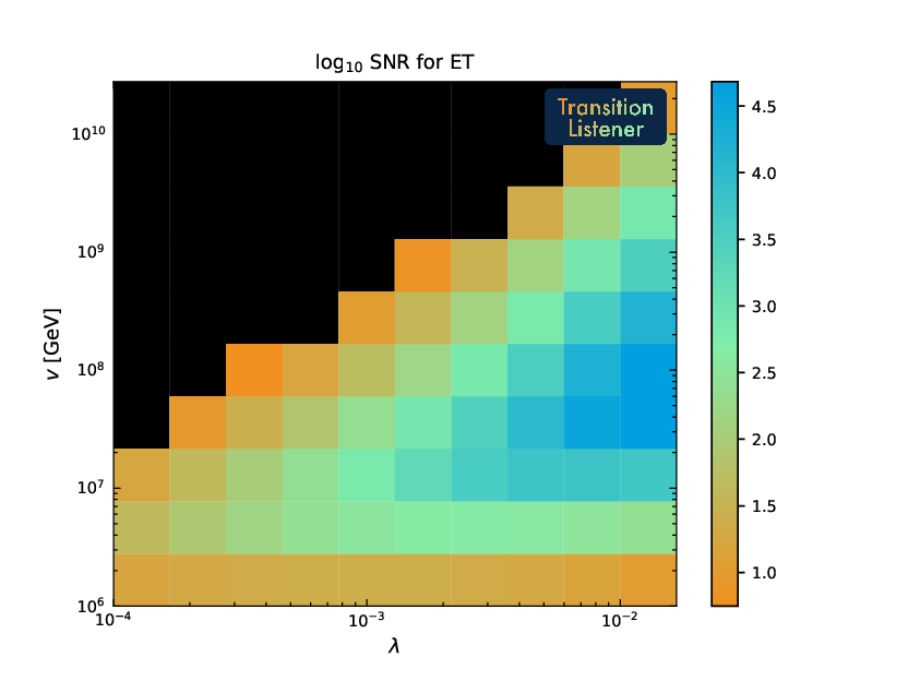
Detector signal-to-noise maps

The final group illustrates how the predicted signals map into the signal-to-noise ratios of selected future detectors.

SNR_BBO	SNR_DECIGO	SNR_ET