Method

The figure below summarizes the end-to-end workflow implemented in TransitionListener.

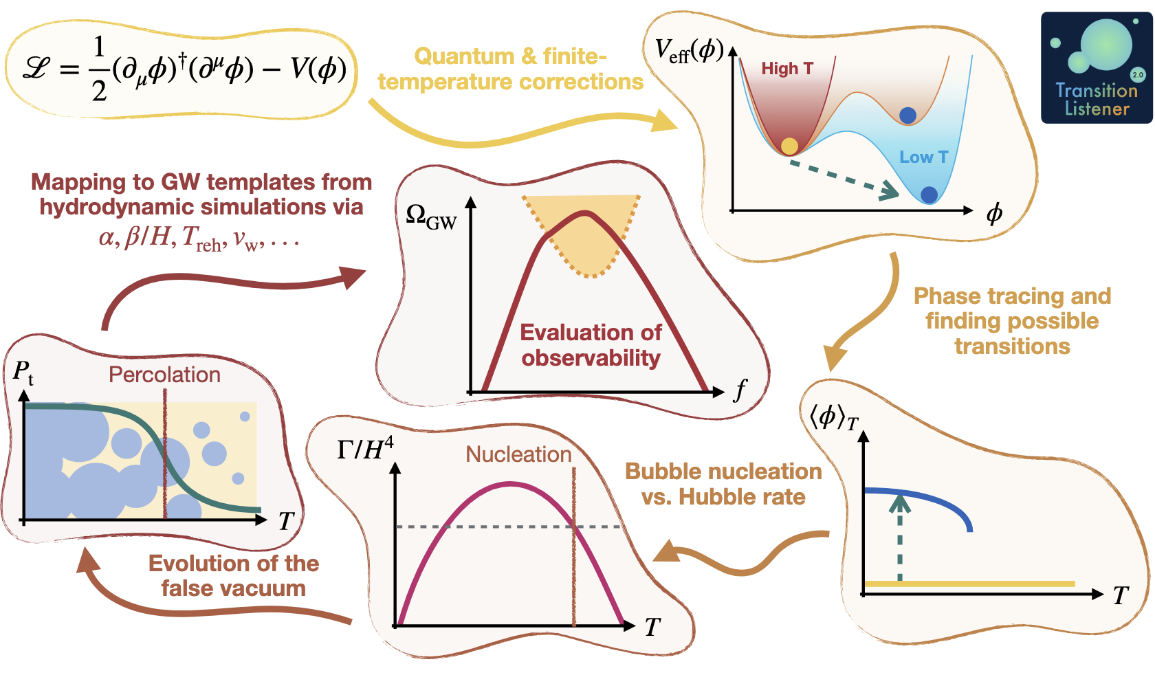
TransitionListener takes a user-defined particle-physics model and turns it into a prediction for the gravitational wave signal of a cosmological first-order phase transition. Internally, the calculation proceeds through a fixed sequence of physics modules coordinated by transitionlistener.interface.pipeline.

From model definition to the effective potential

The starting point is a model file that specifies the tree-level scalar potential, the field content, counterterms, and the field-dependent mass spectrum. In practice, user models inherit from transitionlistener.generic_potential, which provides the common infrastructure for evaluating the effective potential and its derivatives.

At finite temperature, the code constructs the one-loop, daisy-corrected effective potential

\[V(\phi, T) = V_\text{tree}(\phi) + V_\text{CW}(\phi) + V_\text{ct}(\phi) + V_\text{T}(\phi, T) + V_\text{daisy}(\phi, T) + V_\text{rad}(T) - V_{T=0}(v)\,.\]

where \(V_\text{CW}\) is the Coleman-Weinberg correction, \(V_\text{ct}\) contains the counterterms, \(V_\text{T}\) is the finite-temperature contribution, and \(V_\text{daisy}\) is the daisy-resummation term. The thermal integrals \(J_\text{b}\) and \(J_\text{f}\) and the particle bookkeeping are handled through transitionlistener.finiteT, transitionlistener.particles, and transitionlistener.thermodynamics. The code supports the Arnold-Espinosa and Parwani resummation prescriptions through the model configuration.

Phase tracing and transition finding

Once \(V(\phi, T)\) is known, TransitionListener traces all relevant local minima as functions of temperature using transitionlistener.phases. The result is a temperature-ordered phase history that records where phases appear, disappear, or become degenerate.

transitionlistener.transitions then inspects the traced phases and identifies candidate first-order transitions between them. This step determines which pairs of phases coexist over some temperature interval and therefore may be connected by thermal tunnelling. Very weak transitions can be filtered out already at this stage when the vacuum-energy release is too small to be phenomenologically relevant.

Bounce action and nucleation history

For each candidate transition, the tunnelling path in field space is constructed with transitionlistener.pathDeformation. Along this path, TransitionListener evaluates the three-dimensional Euclidean bounce action \(S_3(T)\) using transitionlistener.tunneling1D.

The bounce action determines the thermal bubble-nucleation rate,

\[\Gamma(T) = T^4 \left(\frac{S_3(T)}{2\pi T}\right)^{3/2} \exp\!\left[-\frac{S_3(T)}{T}\right].\]

This quantity enters the nucleation and percolation analysis in transitionlistener.bubbledynamics. The code first builds an initial estimate of the percolation regime and then solves the percolation integral, either with a fixed temperature grid or with an adaptive ODE-based method.

The central quantity is the fraction of space that has converted to the true vacuum,

\[P_\mathrm{t}(T) = 1 - \exp[-I(T)]\,,\]

where \(I(T)\) is the percolation integral. In the final step of the algorithm, TransitionListener iterates this computation self-consistently so that the changing vacuum composition feeds back into the Hubble rate and into the temperature evolution. This is also the stage where reheating and the completion of the transition are determined.

Macroscopic transition observables

After the nucleation history has converged, the module transitionlistener.transitionObservables computes the macroscopic quantities that characterize the phase transition. These include the milestone temperatures such as the nucleation, percolation, final, and reheating temperatures, together with the transition-strength and time-scale measures used in gravitational wave calculations.

The key outputs are the transition strength \(\alpha\), the inverse duration \(\beta/H\), the mean bubble separation \(RH\), and the bubble wall velocity \(v_\mathrm{w}\). Hydrodynamic response and efficiency factors are obtained with transitionlistener.hydrodynamics, while the background thermodynamics relies on the phase-dependent energy density, pressure, and effective relativistic degrees of freedom.

Gravitational wave prediction and observability

The macroscopic observables are then passed to transitionlistener.gwfopt, which evaluates the gravitational wave spectrum from the relevant production channels according to the selected template settings. If several first-order transitions occur, the strongest one is used for the default gravitational wave prediction.

Finally, transitionlistener.observability compares the predicted spectrum to the sensitivity of current and future detectors. This last stage turns the microphysical model input into phenomenological quantities such as signal-to-noise ratios, detector reach, and PTA likelihood-based summaries.