Usage

After pip-installing TransitionListener, you can easily start using it from your terminal. It is really simple to get started.

Configuration files

All it takes is a human-readable configuration file, a .yaml file, which specifies the model parameters, scanning ranges, and desired outputs.

You can find example configuration files in the config/ directory of the TransitionListener repository.

Single point evaluation

Let’s say you have created a configuration file named example_point.yaml in the example/ directory, which specifies a benchmark point which you would like to know of whether it features a first-order phase transition and what gravitational wave signal it produces.

You can run TransitionListener using the command line interface as follows:

$ tl -c examples/example_point.yaml -v

This command will execute TransitionListener with the specified configuration file and enable verbose output. This will print detailed information about the progress of the computation to the terminal. When the computation is finished, the results will be saved to the scans directory to a subfolder as specified in the configuration file. In there you will find various output files, including 0_Input_params.txt reminding you of the chosen input parameters, 1_All_params.txt showing all computed parameters during the performed run, as well as 2_Observability.txt containing the computed observability metrics. Further, additional plots and log files including information about the computation process are saved there.

Grid and line scans

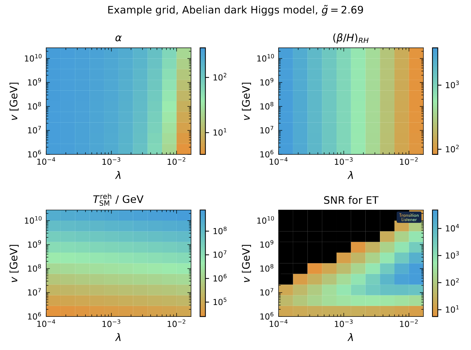
If you want to run a small grid scan using the command line interface, you can use the following command:

$ tl -c examples/example_grid.yaml -j 10

The -j flag specifies the number of parallel jobs to run. Here we took 10 jobs. This can speed up the scan significantly on multi-core machines. The above scan takes a only a couple of minutes on a modern machine. After the scan is complete, the results will be saved in the specified output directory. You will find various output files, including also the following overview plot.

On top of that, you will find close to 200 intermediate results saved in the output directory, in the form of .txt files as well as .pdf plots.

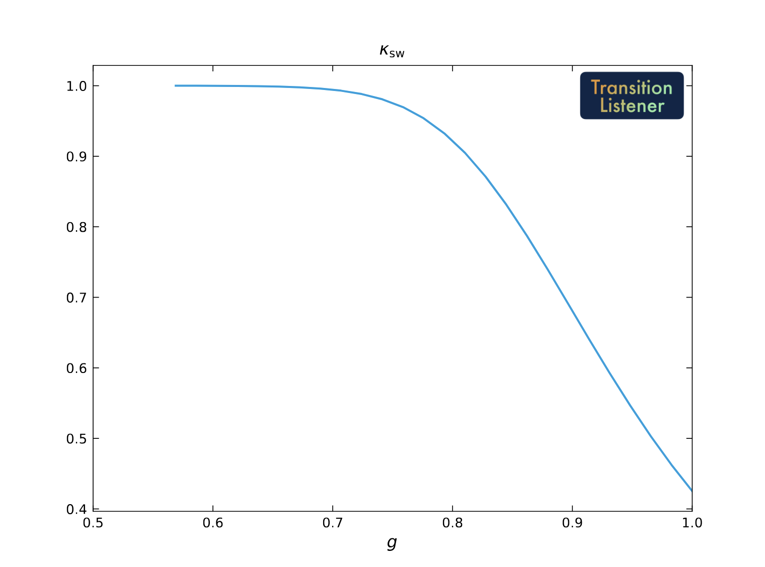
Alternatively, you can also run an example line scan using the following command:

$ tl -c examples/example_line.yaml -j 5

This will perform a line scan over the specified parameter range with 5 parallel jobs. The results will be saved in the output directory as specified in the configuration file. The output is very similar to the grid scan case. For instance, you will find the efficiency factor for converting released vacuum energy to bulk fluid motion among them:

Percolation algorithm controls

TransitionListener exposes two percolation solvers through the configuration:

• adaptive_step_size is the default. It does not require a nucleation- temperature seed and instead builds an adaptive support bank for \(P(T)\) on the fly: the controller scouts the bubble-nucleation-rate peak, protects the high-temperature onset where the bubble nucleation rate is still very small, and then refines the temperature interval in which the true-vacuum fraction increased from zero to one. It further rejects points with unresolved bounce action jitter. The percolation integral is solved via an ODE solver (percolation_integral_method = "ode") using the time-temperature relation in the false vacuum dervied from the speed of sound in that phase.

• fixed_step_size is the an alternative solver of the percolation integral, which sometimes gives more robust results when the adaptive step size solver fails due to numerical instabilities. It evaluates the percolation integral on a precomputed TSYM grid of size percolationConf.n_action (default 30; n_action = 100 gives the high-resolution benchmark setup). As it requries a nucleation temperature as as seed, which first needs to be computed, it is a bit slower on average and cannot deal with cases in which the \(\Gamma = H^4\) condition can never be satisfied, i.e. for extremely slow phase transitions. For most cases, this mode is however a good alternative, in case any unexpected behavior occurs during the percolation computation.

The most important controls are:

• percolation_algorithm_mode: adaptive_step_size or fixed_step_size.

• percolation_integral_method: ode (default) or double_integral for diagnostics.

• percolation_time_temperature_mode: sound_speed (default) uses the symmetric-phase \(c_s^2(T)\) and the cosmological scale-factor ratio \(a(T)/a(T_\mathrm{hot})\) inside the percolation integrand. bag falls back to the \(c_s^2 = 1/3\) limit (no scale-factor weighting).

• percolation_entropy_definition: which entropy fixes the time-temperature relation, and so both the sound speed and the scale factor. dof_table (default) counts the free particles of the traced phase at their zero-temperature masses and adds the tabulated coupled bath; eff_potential takes \(s = -\mathrm{d}V/\mathrm{d}T\) from the effective potential, with thermal masses and the Arnold-Espinosa daisy. Only the adaptive step size solver reads this setting; the fixed step size solver refuses anything but the default, because its time-temperature relation is its own.

• percolation_entropy_scheme_diagnostic and percolation_entropy_scheme_warn_threshold: every adaptive step size run in sound_speed mode compares the two entropy definitions on the percolation support and reports how far apart they are, in DIAG:entropy_scheme_cs2_spread and DIAG:entropy_scheme_lna_gap. The fixed step size solver does not read this setting at all and refuses anything but the default, so it has nothing to compare: it writes the flag as false and both diagnostics as nan. The same combination, a false flag beside two nan, means “not compared” and not “compared and found to agree”; it also arises in bag mode, with the comparison switched off, and where the expansion history could not be built. The first is the median relative difference between the two definitions’ \(3 c_s^2\) over the percolation support, and estimates to about 30% how far the mean bubble separation of that point moves between them. WARNING:entropy_scheme_sensitive is raised when it exceeds the threshold, 4% by default, so a flagged point is one whose \(R_*\) is uncertain at about the five per cent level from this modelling choice alone. Lower the threshold to see weaker cases.

• gwConf.sound_speed: "compute" (the default) takes the sound speed of the plasma from the effective potential; "1/3" uses the massless value \(1/\sqrt{3}\); a number strictly between zero and one is used as \(c_s\) itself. Both percolation solvers accept all three.

  In "compute" mode a value of one or more is refused rather than replaced, with CLI error code 18, for the symmetric phase as well as the broken one: \(c_s\) sets the speed at which the bubbles grow, \(\max(v_\mathrm{wall}, c_s)\), and the spectrum divides by \(v_\mathrm{wall} - c_s\), so a value that is not a speed has no meaning downstream. Which thermodynamics a model has is the user’s choice, so nothing is substituted; set sound_speed to "1/3" or to a number to run such a point anyway. A phase that has simply frozen out, where the ratio is zero over zero or negative, is still reported as nan and is not an error.

• CLI error code 8 is raised from two different stages, and the message says which. While the transition path is being built, it means a candidate reached the nucleation solver and the solve did not succeed, which may be because the transition is too supercooled to nucleate one bubble per Hubble volume or because the solve failed numerically; the error does not distinguish those and says so. Later, during percolation, it means the transition was found and its actions computed but the true vacuum fraction never reached f_perc over the temperature range explored, and the message gives the fraction reached and the lowest temperature tried.

• CLI error code 19, no viable phase pair, comes only from the first of those stages and is the narrower statement: the nucleation solver was never reached, because no pair of phases below the current one was a tunnelling candidate at all. A child never becomes a candidate for one of two reasons, that it duplicates a child already offered or that the two phases do not overlap in temperature. A pair that is evaluated can still be refused, and the counts report that apart: in the adaptive backend a candidate is refused when the starting phase is already the deeper minimum at the cold end of the overlap, when it does not exist to a higher temperature than the target, or when the potential difference could not be evaluated there; on the fixed-step path it can instead fail the nucleation solve. Nothing about the rate was computed, so nothing about supercooling is being claimed. Its message, and the transition-path form of code 8, report how many child phases were listed, how many were evaluated as candidates, and how many ended in a nucleation solve that did not succeed; run with verbose=True to see each phase pair. Those three counts belong to the transition-path stage alone. The percolation form of code 8 carries none of them, because at that point the transition has already been found; it reports the fraction reached and the lowest temperature tried, as above. So a scan reading code 8 should take the counts as present only when the message is the transition-path one.

• WARNING:noisy_c_s and DIAG:c_s_step_change: whether the computed sound speed survives a change of the derivative step. A value can be round-off and still lie between zero and one, so no test on the value itself finds it; the step is varied by a factor ten in each direction and the larger relative change is reported, with the warning raised above 5%. On a healthy point the change is of order \(10^{-7}\). A value that is refused at one test step and not at another is noisy, because it stopped being a speed somewhere inside the step range and no single step shows that; one refused at every step is not, since it does not depend on the step and the refusal itself already reports it. nan means the change could not be put as a ratio, which happens when the value does not exist at one of the steps or is infinite at all of them.

• WARNING:daisy_outside_validity and DIAG:daisy_over_radiation: whether the Arnold-Espinosa daisy resummation is being used where it does not apply. That term resums the bosonic zero Matsubara mode, which is justified for \(m \ll T\). For \(m \gg T\) a mode should be Boltzmann suppressed, and the one-loop thermal integral is; the daisy term is not, going instead as a power of the temperature. Where it dominates, the free energy goes as \(T^3\) rather than \(T^4\) and \(c_s^2\) drifts towards \(1/2\) instead of the \(1/3\) of radiation. The diagnostic is the ratio of the daisy term to the field-independent radiation, and the warning is raised when that exceeds one and the lightest mode has \(m/T > 1\); both are needed, because at high temperature a large ratio is legitimate. This reports a modelling choice, not an error, and nothing is corrected. It applies only to daisy = "ArnoldEspinosa"; with "Parwani" or "off" there is no such term in the potential and both come back as a false flag beside a nan.

  The daisy term itself needs the thermal part of the boson masses, \(\Pi\). Where a model writes its Debye masses in closed form it should override generic_potential.debye_massSq; otherwise the base class measures them, by reading the \(T^2\) coefficient off the model’s own spectrum at a temperature where the difference of the spectra still keeps its digits. That the thermal part is quadratic is verified rather than assumed, and the base class falls back to the difference of the two spectra wherever it is not. It is not, for every model whose bosonic masses are eigenvalues of a mass matrix that mixes: the entries of such a matrix go as \(T^2\) but its eigenvalues do not. Of the models shipped in models/, the two dark \(U(1)\) parameterisations, the conformal dark \(U(1)\) and the template get an exact \(\Pi\), while the three 2HDM models and the dark flip-flop use the difference.

  A model that rewrites the effective potential must override generic_potential.V_thermal as well as Vtot and V1T_from_X. It returns the temperature-dependent part on its own, including the radiation bath its include_decoupled argument selects, and the sound speed, the transition strengths and the wall velocity are all taken from it. Overriding Vtot or V1T_from_X without it raises errors.PotentialError: those two differ in whether they carry the bath and the daisy term, so neither can be used to stand in for it, and reconstructing one from the mass spectrum would not be the model’s own.

• percolationConf.n_action: fixed TSYM support count for fixed_step_size runs.

• percolation_n_action_min, percolation_n_action_increment, percolation_n_action_max, percolation_max_action_temperatures, percolation_maxit: support-bank controls for adaptive_step_size.

• percolation_jitter_GH4_threshold: the bounce-rate jitter detector (in \(\log_{10}(\Gamma/H^4)\)) – default 1.0; raise to 2.0 or so on models with very steep, deeply supercooled action profiles.

• percolation_max_log10_rate_step: largest change of \(\log_{10}(\Gamma/H^4)\) allowed between neighbouring support points – default 12.0. Intervals above it are refined before jumps in \(P\), because the percolation integral interpolates the logarithm of the rate and cannot resolve a rise that happens inside one interval. Zero switches the criterion off.

• percolation_acc_tperc, percolation_acc_tfinal, percolation_acc_rh: refinement and stopping controls for adaptive_step_size.

All of these can be set globally in the YAML configuration or directly in a model file via setConfigParameters() when model-specific defaults are desired. The default configuration uses adaptive_step_size with the ode / sound_speed integral, so most users do not need to touch any of these knobs.

Precision modes

The tracing and tunnelling precision presets are configurable through precision_mode:

• default – vanilla settings.

• robust – tighter phase tracing only.

• xtrace – still tighter tracing (very small dtstart, dtmin).

• tunneltight – default tracing plus tighter bounce path-deformation tolerances.

• benchmark – tightens both tracing and tunnelling. Note: While being the most precise mode, it can be computationally expensive, with runtimes of a single computation of over one hour, in the case of multi-dimensional scalar potentials.

Radiation baths

Radiation that is not part of the potential belongs to one of two baths, set in the model’s init:

• kin_coupled_e_geff and kin_coupled_p_geff (default: the Standard Model) describe radiation in thermal contact with the fields of the potential. Together they form the transitioning sector, which is reheated inside the bubbles.

• kin_decoupled_e_geff and kin_decoupled_p_geff (default: empty) describe radiation that is not. It is not reheated inside the bubbles, keeps the temperature of the surrounding false vacuum and enters the expansion rate and the redshift of the gravitational-wave spectrum. With pot.config.gwConf.coupled_hydrodynamics = True (the default) it also moves with the fluid and enters the hydrodynamics and the strength alpha.

For a dark sector decoupled from the Standard Model, move e_geffSM and p_geffSM from the coupled to the decoupled bath, set the coupled bath to zero, and set pot.config.gwConf.coupled_hydrodynamics = False, so that the Standard Model does not enter the hydrodynamics either. TL takes the bath whose tables are e_geffSM as the Standard Model bath; if the tables are wrapped, set self.SM_bath = "decoupled" (or "coupled") in the model. It warns if both baths hold e_geffSM. A model whose potential contains Standard Model fields (flagged is_SM, e.g. the 2HDM) has the Standard Model in its transitioning sector; TL then refuses a decoupled Standard Model, while other radiation, e.g. of a dark sector, can still go into the decoupled bath.

Both baths share the temperature before the transition, so Tnuc_SM_GeV and Tperc_SM_GeV apply to both. Treh_SM_GeV is the temperature of the Standard Model bath at reheating, which happens at percolation: the reheated temperature if the Standard Model is coupled, Tperc if it is decoupled. Treh_DS_GeV is the reheating temperature of the transitioning sector. g_eff_tot_reh and h_eff_tot_reh sum the fields of the potential, the coupled bath and the decoupled bath, each weighted by its temperature ratio to the Standard Model bath to the fourth and third power. The redshift assumes that the energy and entropy of the dark sector end up in the photon bath without entropy injection (dilution factor D = 1). Two simplifications apply: the decoupled bath is evaluated at the temperature of the transitioning sector until the transition, although the two can drift apart where the degrees of freedom of either change, and the evolution of the temperature ratio after the transition is not modelled. For the same reason a decoupled bath is only consistent for the first of several transitions: after it, the bath is colder than the transitioning sector.

Random and nested sampling scans

You can also run a random scan by using the following command:

$ tl -c examples/example_random_conformal.yaml -j 10

This will perform a random scan over the specified parameter ranges with 10 parallel jobs. The results will be saved in the output directory in a .csv file. You can use this file to analyze the results further or visualize them using your preferred plotting tools.

If you are interested in performing a nested sampling scan using mpi for parallelization you can use the following command:

$ mpiexec -n 16 tl -c config/example-nested-scan.yaml

This will run a nested sampling scan with 16 parallel processes. The results will again be saved in a .csv file in the specified output directory.

For detailed installation instructions and usage examples please refer to the following sections:

• Installation: Installation Guide

• Usage: Usage

For more information, visit the documentation at https://tasillo.de/TransitionListener_development or check out the code repository at https://github.com/tasicarl/TransitionListener.